go to Table of Contents

Wavelet Theory Why Wavelets Are Good For Image Compression

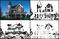
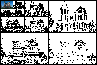
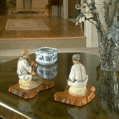
THE POWER OF MATHEMATICS Until the mid 1960's the Fourier transform was usually numerically computed using the discrete Fourier transform (DFT): 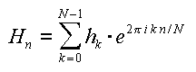here n = -N / 2 ... N / 2 and h k are the N signal data points ( k = 0 .. N - 1 ). The value of the DFT is that it decomposes a signal into frequency components (sine and cosine waves). On the frequency side many things about the input signal can be discovered, such as cyclic reoccurrence of events, and some complicated operations, such as convolution, can be reduced to simple multiplication. Frequency bandpass operations allow noise removal and allow information etched on a carrier signal to be extracted from it. Due to its usefulness in all areas of engineering, science, and mathematics, a quick way to compute it was needed. Using the formula above, it is easy to calculate how many additions and multiplications are required to transform a signal into its frequency components. Given a signal of length N, we see that it takes N x N multiplications to compute the DFT. Anyone who has performed a runtime analysis on a computer algorithm immediately understands that an N x N runtime can bog down the most powerful computer. Suppose the input signal is 106=1,000,000 data points long, a microscopic input relative to digital video and sound. To transform this tiny signal into the frequency domain using the DFT requires at least 106 x 106 multiplications. On a 486 it takes 16 clock cycles to perform 1 floating point multiplication. So it will take at least 16 x 1012 clock cycles just to perform the multiplications. How fast is this? If your computer's cpu speed is 100 MHz = 10 x 107, then the time spent on multiplying is (16 x 1012) / (10 x 107) = 1.6 x 105 secs = 44.4 hours = 1.85 days. Keep in mind that one frame from a digitized video sequence can easily contain 1,000,000 pixels. In the mid 1960's (even though it was known years earlier) a method for computing the DFT which has a runtime of N x log2(N), the famous FFT (fast Fourier transform), was published, popularizing its use. How important is the FFT? The number of multiplications is reduced to 106 x 19.9 which yields a runtime of (19.9 x 106) / (10 x 107) = 0.199 secs. Isn't that incredible? Although there are applications where the Fourier transform is the ideal tool, there are others where one of its properties is a severe drawback, that of giving global frequency information. For instance, given a sound signal composed of two tones played one after the other, the Fourier transform only reveals the tones but not the order in which they occur. The simultaneous mapping of time and frequency can never be completely achieved due to the Heisenberg uncertainty principle. Nevertheless, people pressed on with their search for an optimal balance between the time and frequency domains. In the mid 1970's, built upon the Littlewood-Paley theories, mathematicians worked out a near optimal solution to this time/frequency dilemma. From there orthogonal solutions appeared creating simple invertible transforms. In the early 1980's, all of these theories converged into wavelet theory. Today, through the work of many researchers, the wavelet transform has become a powerful tool in signal and information analysis due to its ability to simultaneously identify frequency (or scale) components and their locations. Most remarkably of all, its runtime is directly proportional to the length of the input signal and thus requires only N multiplications (times a small constant) to compute the transform. In terms of computer science, you cannot do much better than that. THE POWER OF WAVELETS Time / frequency localization achieves the immediate benefit of information condensing. This, perhaps more than any other capability, is where the power of wavelets lie. The wavelet transform reduces information in a signal roughly to averages and differences of neighboring pixels at discrete scale (frequency) levels. In an image, the information in areas of near constant color (a blue sky for instance) is collapsed into the average component and the difference components are close to zero. Each average and difference component contains information about an area 4 times as big as it. If the differences are close to zero you can throw them away and all the information about the area is contained in the average components. This is why the wavelet transform is naturally linked to digital image compression. Below is an image and its wavelet transform (after thresholding) illustrating the information condensing property. 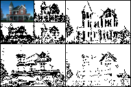original wavelet transform same size blocks = same scale (frequency) level red = non-zero wavelet coeffiecents Just as with the Fourier transform, a fast version of the wavelet transform has been devised. It is called the fast wavelet transform (FWT). Summus' version of the FWT transforms digitized data into the frequency domain blindingly fast. The sequence below shows the progress of an image being transformed through the frequency levels. 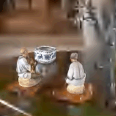original 1 level 2 levels 3 levels Flexibility is another characteristic that makes the wavelet transform an important tool in this age of communication. The FWT lends itself ideally to applications which require reordering of digital information. Its adaptability is easiest seen in the progressive transmission of an image over a digital data link. The image sequence below shows information in a wavelet compressed image being decompressed according to a user defined ordering. 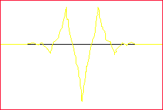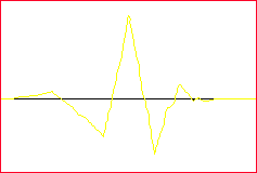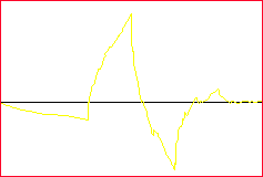time 1 decomp basic content time 2 decomp bowl time 3 decomp figures time 4 deomp background The power behind wavelet data reordering (besides the obvious usefulness of the capability) is that incoming information builds on that already received, resulting in no computational or information overhead. In other words the time and information it takes to decompress an image piecewise is the same as decompressing the image all at once. If you have read this far you are no doubt asking yourself, "what do wavelets look like?". There are literally an infinite number of wavelets in any dimension that you like, 1 dimensional, 2 dimensional, 3 ..., N dimensional. Only 1, 2, and 3 dimensional are of practical use and among these only a handful are of significant value. Image compression uses 2 dimensional wavelets, video compression may use 3 dimensional ones, and signals such as sound can be analyzed using 1 dimensional wavelets. Below are a few wavelet graphs. If you would like to learn more about the theory of wavelets the following references are a good place to start: Ten Lectures on Wavelets by I. Daubechies Recent Advances in Wavelet Analysis edited by L. Schumaker and G. Webb [ The Wavelet Digest ] If you are developing an application that requires image or video compression and would like more information about Summus' compression products, please feel free to call us or fill out our [ Contact ] page and we will be glad to assist you.